Making Git prompt for SSH username

In what seems to be an unusual configuration—as I was unable to find any information on how to do it—I had a need to make Git prompt for an SSH username. The repositories in question are on a shared computer, but the host for the remote copies requires individual user authentication using a password and a TOTP code. A crude solution was to set GIT_SSH_COMMAND='ssh -l $USER', but this requires the user to remember to run, e.g., USER=username git pull, although this can be helped by setting USER='Prefix_git_with_"USER=yourusername"!!!!!!!!' in .bashrc. After much trial and error, I arrived at the solution of setting the GIT_SSH environment variable in .bashrc to point at the following shell script:

#!/bin/bash
# Make Git prompt for SSH username
# M. Petroff, 2024-12
if [[ $1 = "-G" ]]
then
  # Handle Git's SSH variant test
  ssh "$@"
else
  # Prompt for username
  read -p "Username: " user </dev/tty
  ssh -l "$user" "$@"
fi

There are two peculiarities here to keep in mind. First, stdin and stdout cannot be used, so input redirection needs to be used with read to get input directly from the terminal (/dev/tty), similar to what SSH itself does; with the -p flag, read writes to stderr, which is okay. With this resolved, there were mysterious issues with either the username prompt being displayed twice or with needing to press “enter” to see the prompt, depending on the exact details of the then work-in-progress script. I eventually realized this was due to Git’s SSH variant checking, which first calls the GIT_SSH command with the -G argument to figure out which variant of SSH is in use. While this check can be avoided by setting GIT_SSH_VARIANT explicitly, it was easy enough to handle the check in the shell script.

Posted in | Tagged , , , | Leave a comment

2024 Total Solar Eclipse and Mount Bigelow

Early Monday morning, my brother and I drove north from the Boston area to Maine for the total solar eclipse. Originally, we had planned to view the eclipse from New York, in the Adirondacks, but, a few days prior, the cloud forecast for Maine was looking much better.1 The goal in either case was to climb above the tree line for the eclipse, and with clouds in the forecast for New York, the Vermont peaks being closed for mud season, and the New Hampshire high peaks being too far south, that left Maine. We considered both Mt. Abraham and Mt. Bigelow, before deciding on Mt. Bigelow for its easier access and longer period of totality.

Leaving around 4 am, we encountered no traffic until shortly before reaching our destination, the Bigelow Preserve, where we were stuck in stop-and-go traffic for 15–20 minutes; the traffic was trying to turn into the access road for the Sugarloaf ski resort, which was backed up. Due to a lack of winter road maintenance on Stratton Brook Pond Road, we parked on ME-27, where the Appalachian Trail crosses it; as it was a busy day on the trail, the parking lot was full, and we parked on the side of the road. We started hiking shortly after 9 am carrying our snowshoes but quickly decided to put them on. There appeared to be at least a foot of snow on the ground, and the trail was a bit icy at this point, with a satisfying crunching noise while walking, although the snow became much softer as the day went on and temperatures rose well above freezing. When the Appalachian Trail started to climb the mountain, which was quite steep at times, the several layers we were wearing became much too warm, and we both stripped down to just a t-shirt for the remainder of the climb.

Continue reading


  1. I was carefully checking both the ECMWF cloud forecast online and loading the NWS National Blend of Models into QGIS, with roads, borders, and the region of totality overlaid. 

Posted in , | Tagged , , , , , , | Leave a comment

Antarctica and the South Pole

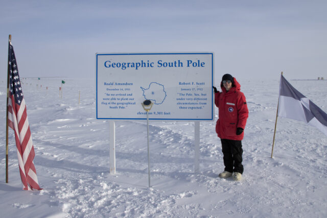
This past austral summer, I was fortunate enough to be able to spend two months in Antarctica working on the BICEP / Keck telescopes under the United States Antarctic Program (USAP).1 Due to limited deployment slots, I was originally on a list of alternates, who also completed the rigorous physical qualification (PQ) process, and found out that I would deploy shortly before Thanksgiving—roughly two weeks before I left—after a slot opened up on the primary deployment roster.

Large white "Geographic South Pole" sign installed in snow with person wearing red parka standing next to it and metal Geographic South Pole marker in front of it. Continue reading


  1. And, yes, I got back almost six month ago and am just writing this blog post now. 

Posted in | Tagged , , , , , | Leave a comment

BICEP Cookies

Earlier this week, this year’s BICEP / Keck collaboration meeting was held at Harvard (we build, operate, and analyze data from cosmic microwave background telescopes installed at the South Pole). As a collaboration member at the host institution, I decided to bake some BICEP-themed cookies for a coffee break at the meeting, arriving at the idea of making butter cookies in the style of Pepperidge Farm Chessmen cookies.

A dozen butter cookies arranged in a grid on parchment paper, with E- and B-mode polarization patterns, Antarctica themes, and BICEP themes as raised designs Continue reading

Posted in , | Tagged , , , , , | Leave a comment

An Improved CMB Map Colormap

Although a variety of colormaps have previously been specifically developed for displaying cosmic microwave background (CMB) maps, none of these have been designed with perceptual uniformity or color-vision-deficiency (CVD) accessibility in mind. To improve upon this status quo, in support of publications1 for the 2022 data release for the Cosmology Large Angular Scale Surveyor (CLASS), I used Matplotlib’s Viscm tool to develop a new diverging colormap that resembles the Planck colormap but is mostly perceptually uniform and is perceived similarly by both individuals with typical color vision and those with red or green color-vision deficiencies. The Q-band Stokes U map from the CLASS paper, which uses the new colormap, is shown below.

A CMB map in equatorial coordinates is shown under Mollweide projection. Data are shown for around 70% of the sky, and the Galactic plane is visible. The new colormap discussed in this blog post is used, starting from blue to a warm light gray and then to red. Continue reading


  1. Y. Li et al., “CLASS Data Pipeline and Maps for 40 GHz Observations through 2022”, arXiv:2305.01045.  

Posted in | Tagged , , , , | Leave a comment